In this tutorial, we’ll explore how to perform data standardisation and normalisation in R. These preprocessing steps are critical for many statistical analyses and machine learning models, as they can significantly impact performance and results.
41.1 What are Standardisation and Normalisation?
Standardisation (also known as Z-score normalisation) is the process of rescaling the features so they have the properties of a standard normal distribution with a mean of 0 and a standard deviation of 1.
Normalisation typically means rescaling the values into a range of [0, 1].
41.2 When are they used?
You would standardise your data when you need to compare features that have different units or scales, particularly in models that assume normally distributed data, such as linear regression, or when using techniques that are sensitive to variance, like principal component analysis (PCA).
Standardisation is useful because it transforms your data to have a mean of 0 and a standard deviation of 1, ensuring that each feature contributes equally to the analysis.
On the other hand, normalisation is used when you need to bound your data within a specific range, such as [0, 1], which is often required by algorithms that assume data is in a bounded interval, like neural networks, or when you’re working with models that use distance calculations, such as k-nearest neighbours (KNN).
Normalisation helps in speeding up the convergence of gradient descent algorithms by ensuring all parameters are on a similar scale.
We’ll return to normalisation when covering machine learning later in the module.
41.3 Example
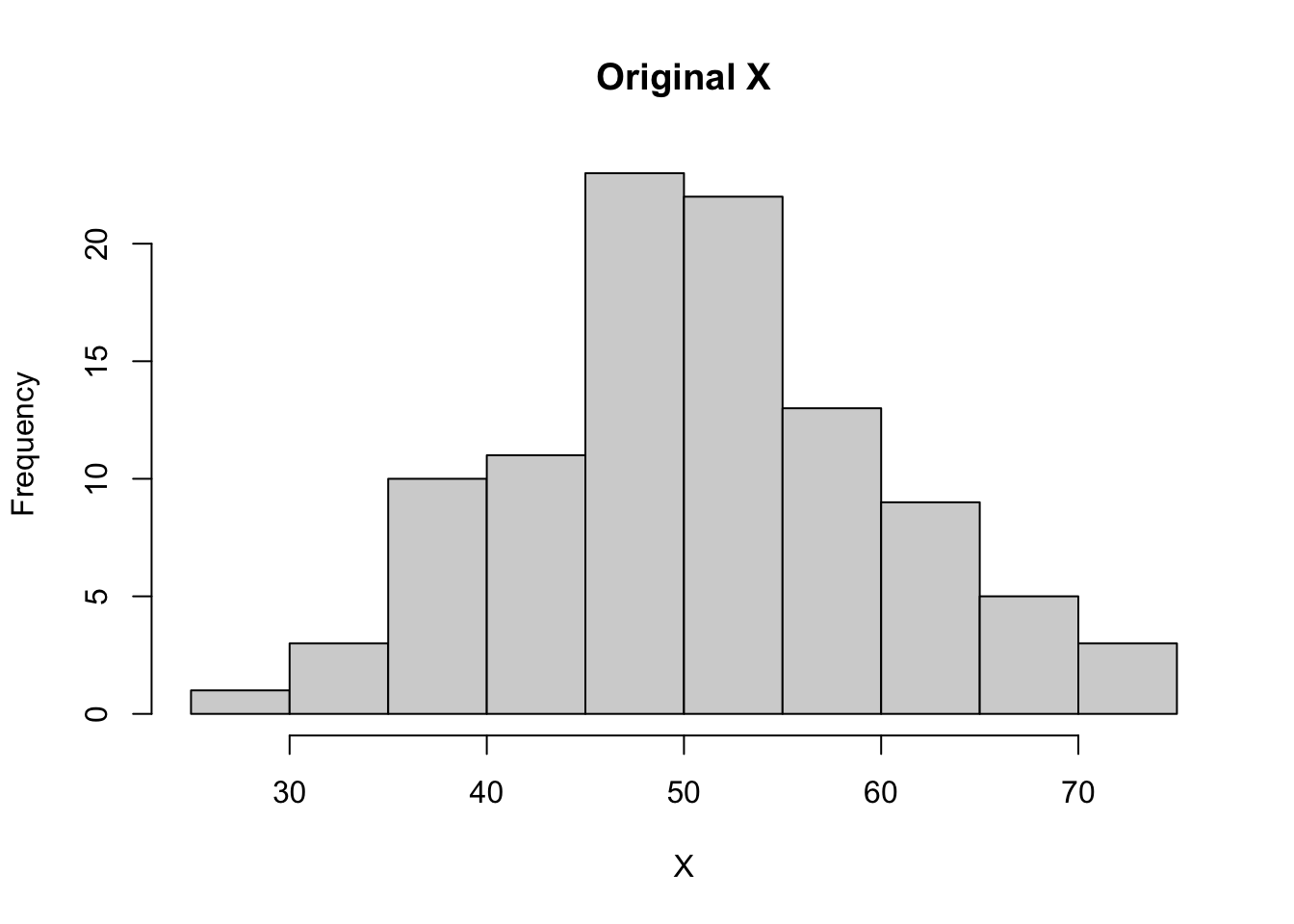
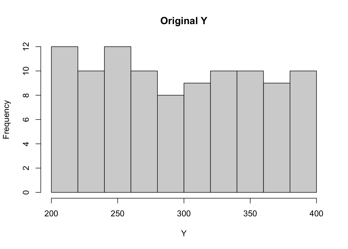
We’ll start by creating two vectors X and Y. X has a normal distribution, and Y has a uniform distribution.
Show code
rm(list=ls())set.seed(123) # Ensure reproducibility# Generate synthetic datadata <-data.frame(X =rnorm(100, mean =50, sd =10), # Normally distributed dataY =runif(100, min =200, max =400) # Uniformly distributed data)# Original Datahist(data$X, main ="Original X", xlab ="X")
Show code
hist(data$Y, main ="Original Y", xlab ="Y")
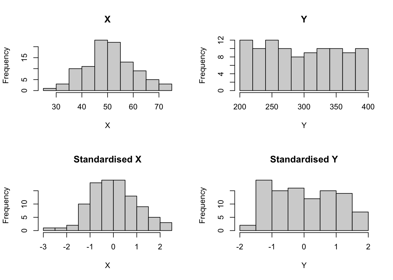
We can standardise the data by using the scale() function. This gives a mean of 0 and SD of 1 for each variable.
Show code for standardisation
library(psych)# Standardise datadata_standardised <-as.data.frame(scale(data))# Summary to verify standardisationdescribe(data_standardised) # using the psych library
  vars   n mean sd median trimmed  mad   min  max range skew kurtosis  se
X    1 100    0  1  -0.03   -0.01 0.97 -2.63 2.30  4.93 0.06    -0.22 0.1
Y    2 100    0  1  -0.04   -0.01 1.27 -1.63 1.69  3.32 0.08    -1.28 0.1
Notice that both variables now have a mean of 0, and a SD of 1.
Show code for plotting
# Plottingpar(mfrow =c(2, 2))# Original Datahist(data$X, main ="X", xlab ="X")hist(data$Y, main ="Y", xlab ="Y")# Standardised Datahist(data_standardised$X, main ="Standardised X", xlab ="X")hist(data_standardised$Y, main ="Standardised Y", xlab ="Y")
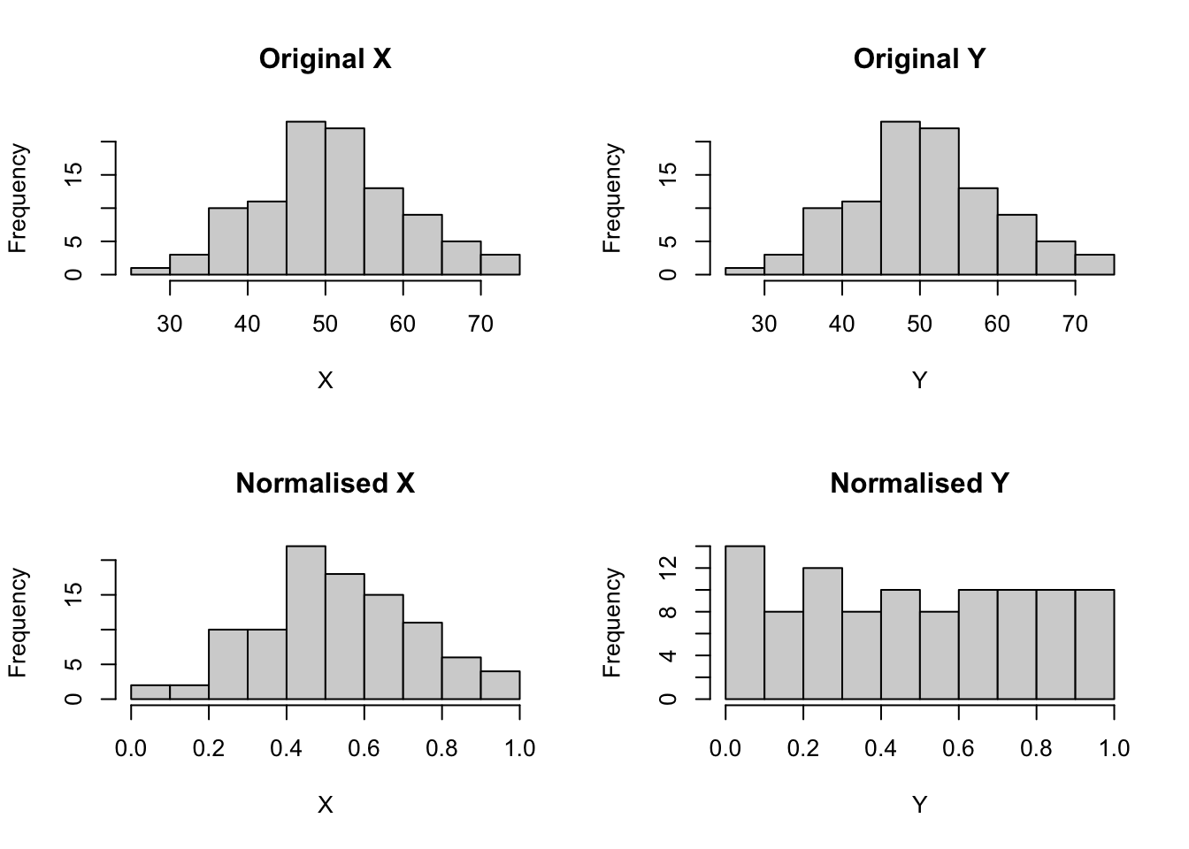
We can also normalise the original data. This scales each variable to a range between 0 and 1.
Show code for normalisation
# Normalize data functionnormalise <-function(x) { (x -min(x)) / (max(x) -min(x))}# Apply normalisationdata_normalised <-as.data.frame(lapply(data, normalise))# Summary to verify normalisationdescribe(data_normalised)
  vars   n mean  sd median trimmed  mad min max range skew kurtosis   se
X    1 100 0.53 0.2   0.53    0.53 0.20   0   1     1 0.06    -0.22 0.02
Y    2 100 0.49 0.3   0.48    0.49 0.38   0   1     1 0.08    -1.28 0.03
Show code for plotting
# Plottingpar(mfrow =c(2, 2))# Original Datahist(data$X, main ="Original X", xlab ="X")hist(data$X, main ="Original Y", xlab ="Y")# Normalised Datahist(data_normalised$X, main ="Normalised X", xlab ="X")hist(data_normalised$Y, main ="Normalised Y", xlab ="Y")
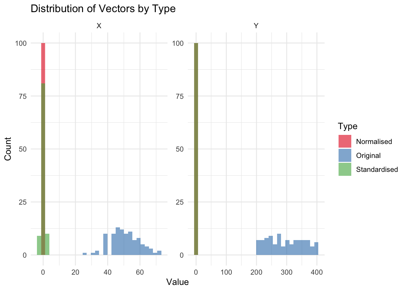
Further visualisations:
Show code for visualisations
library(ggplot2)library(reshape)# Add a 'Type' column to each datasetdata$Type <-'Original'data_standardised$Type <-'Standardised'data_normalised$Type <-'Normalised'# Combine the datasetscombined_data <-rbind(data, data_standardised, data_normalised)# Melt the combined data for ggplot2library(reshape2)data_melted <-melt(combined_data, id.vars ='Type', variable.name ='Vector', value.name ='Value')# Distribution plotsggplot(data_melted, aes(x = Value, fill = Type)) +geom_histogram(alpha =0.6, position ="identity", bins =30) +facet_wrap(~Vector, scales ='free') +theme_minimal() +scale_fill_brewer(palette ="Set1") +labs(title ="Distribution of Vectors by Type", x ="Value", y ="Count")
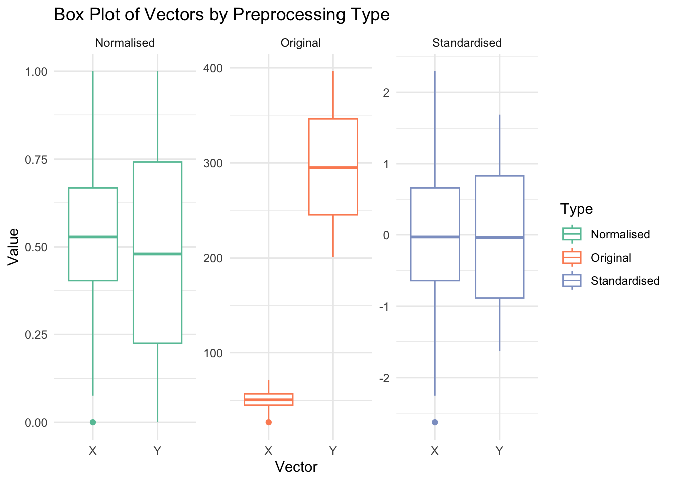
Show code for visualisations
# Box plotsggplot(data_melted, aes(x = Vector, y = Value, color = Type)) +geom_boxplot() +facet_wrap(~Type, scales ='free') +theme_minimal() +scale_color_brewer(palette ="Set2") +labs(title ="Box Plot of Vectors by Preprocessing Type", x ="Vector", y ="Value")